Online Learning in Online Auctions

Dynamics in markets

$$ \def\de{\mathrm{d}} \def\De{\mathrm{D}} \def\x{\times} \def\ve{\varepsilon} \def\dre{\delta r^\ve} \def\de{\mathrm{d}} \def\De{\mathrm{D}} \def\x{\times} \def\ve{\varepsilon} \def\dre{\delta r^\ve} \def\1{\mathbb{1}} \def\argmax{\mathrm{arg}\max} $$ $$ \def\Ab{\mathbb{A}} \def\Bb{\mathbb{B}} \def\Cb{\mathbb{C}} \def\Db{\mathbb{D}} \def\Eb{\mathbb{E}} \def\Fb{\mathbb{F}} \def\Hb{\mathbb{H}} \def\Gb{\mathbb{G}} \def\Ib{\mathbb{I}} \def\Jb{\mathbb{J}} \def\Lb{\mathbb{L}} \def\Kb{\mathbb{K}} \def\Mb{\mathbb{M}} \def\Nb{\mathbb{N}} \def\Ob{\mathbb{O}} \def\Pb{\mathbb{P}} \def\Qb{\mathbb{Q}} \def\Rb{\mathbb{R}} \def\Sb{\mathbb{S}} \def\Tb{\mathbb{T}} \def\Ub{\mathbb{U}} \def\Vb{\mathbb{V}} \def\Wb{\mathbb{W}} \def\Xb{\mathbb{X}} \def\Yb{\mathbb{Y}} \def\Zb{\mathbb{Z}} $$ $$ \def\Ac{\mathcal{A}} \def\Bc{\mathcal{B}} \def\Cc{\mathcal{C}} \def\Dc{\mathcal{D}} \def\Ec{\mathcal{E}} \def\Fc{\mathcal{F}} \def\Hc{\mathcal{H}} \def\Gc{\mathcal{G}} \def\Ic{\mathcal{I}} \def\Jc{\mathcal{J}} \def\Lc{\mathcal{L}} \def\Kc{\mathcal{K}} \def\Mc{\mathcal{M}} \def\Nc{\mathcal{N}} \def\Oc{\mathcal{O}} \def\Pc{\mathcal{P}} \def\Qc{\mathcal{Q}} \def\Rc{\mathcal{R}} \def\Sc{\mathcal{S}} \def\Tc{\mathcal{T}} \def\Uc{\mathcal{U}} \def\Vc{\mathcal{V}} \def\Wc{\mathcal{W}} \def\Xc{\mathcal{X}} \def\Yc{\mathcal{Y}} \def\Zc{\mathcal{Z}} $$ $$ \def\Ar{\mathrm{A}} \def\Br{\mathrm{B}} \def\Cr{\mathrm{C}} \def\Dr{\mathrm{D}} \def\Er{\mathrm{E}} \def\Fr{\mathrm{F}} \def\Hr{\mathrm{H}} \def\Gr{\mathrm{G}} \def\Ir{\mathrm{I}} \def\Jr{\mathrm{J}} \def\Lr{\mathrm{L}} \def\Kr{\mathrm{K}} \def\Mr{\mathrm{M}} \def\Nr{\mathrm{N}} \def\Or{\mathrm{O}} \def\Pr{\mathrm{P}} \def\Qr{\mathrm{Q}} \def\Rr{\mathrm{R}} \def\Sr{\mathrm{S}} \def\Tr{\mathrm{T}} \def\Ur{\mathrm{U}} \def\Vr{\mathrm{V}} \def\Wr{\mathrm{W}} \def\Xr{\mathrm{X}} \def\Yr{\mathrm{Y}} \def\Zr{\mathrm{Z}} $$ $$ \def\ar{\mathrm{a}} \def\br{\mathrm{b}} \def\cr{\mathrm{c}} \def\dr{\mathrm{d}} \def\er{\mathrm{e}} \def\fr{\mathrm{f}} \def\hr{\mathrm{g}} \def\gr{\mathrm{h}} \def\ir{\mathrm{i}} \def\jr{\mathrm{j}} \def\kr{\mathrm{k}} \def\lr{\mathrm{l}} \def\mr{\mathrm{m}} \def\nr{\mathrm{n}} \def\or{\mathrm{o}} \def\pr{\mathrm{p}} \def\qr{\mathrm{q}} \def\rr{\mathrm{r}} \def\sr{\mathrm{s}} \def\tr{\mathrm{t}} \def\ur{\mathrm{u}} \def\vr{\mathrm{v}} \def\wr{\mathrm{w}} \def\xr{\mathrm{x}} \def\yr{\mathrm{y}} \def\zr{\mathrm{z}} $$ $$ \def\As{\mathscr{A}} \def\Bs{\mathscr{B}} \def\Cs{\mathscr{C}} \def\Ds{\mathscr{D}} \def\Es{\mathscr{E}} \def\Fs{\mathscr{F}} \def\Hs{\mathscr{H}} \def\Gs{\mathscr{G}} \def\Is{\mathscr{I}} \def\Js{\mathscr{J}} \def\Ls{\mathscr{L}} \def\Ks{\mathscr{K}} \def\Ms{\mathscr{M}} \def\Ns{\mathscr{N}} \def\Os{\mathscr{O}} \def\Ps{\mathscr{P}} \def\Qs{\mathscr{Q}} \def\Rs{\mathscr{R}} \def\Ss{\mathscr{S}} \def\Ts{\mathscr{T}} \def\Us{\mathscr{U}} \def\Vs{\mathscr{V}} \def\Ws{\mathscr{W}} \def\Xs{\mathscr{X}} \def\Ys{\mathscr{Y}} \def\Zs{\mathscr{Z}} $$ $$ \def\Abf{\mathbf{A}} \def\Bbf{\mathbf{B}} \def\Cbf{\mathbf{C}} \def\Dbf{\mathbf{D}} \def\Ebf{\mathbf{E}} \def\Fbf{\mathbf{F}} \def\Hbf{\mathbf{H}} \def\Gbf{\mathbf{G}} \def\Ibf{\mathbf{I}} \def\Jbf{\mathbf{J}} \def\Lbf{\mathbf{L}} \def\Kbf{\mathbf{K}} \def\Mbf{\mathbf{M}} \def\Nbf{\mathbf{N}} \def\Obf{\mathbf{O}} \def\Pbf{\mathbf{P}} \def\Qbf{\mathbf{Q}} \def\Rbf{\mathbf{R}} \def\Sbf{\mathbf{S}} \def\Tbf{\mathbf{T}} \def\Ubf{\mathbf{U}} \def\Vbf{\mathbf{V}} \def\Wbf{\mathbf{W}} \def\Xbf{\mathbf{X}} \def\Ybf{\mathbf{Y}} \def\Zbf{\mathbf{Z}} $$ $$ \def\abf{\mathbf{a}} \def\bbf{\mathbf{b}} \def\cbf{\mathbf{c}} \def\dbf{\mathbf{d}} \def\ebf{\mathbf{e}} \def\fbf{\mathbf{f}} \def\hbf{\mathbf{g}} \def\gbf{\mathbf{h}} \def\ibf{\mathbf{i}} \def\jbf{\mathbf{j}} \def\kbf{\mathbf{k}} \def\lbf{\mathbf{l}} \def\mbf{\mathbf{m}} \def\nbf{\mathbf{n}} \def\obf{\mathbf{o}} \def\pbf{\mathbf{p}} \def\qbf{\mathbf{q}} \def\rbf{\mathbf{r}} \def\sbf{\mathbf{s}} \def\tbf{\mathbf{t}} \def\ubf{\mathbf{u}} \def\vbf{\mathbf{v}} \def\wbf{\mathbf{w}} \def\xbf{\mathbf{x}} \def\ybf{\mathbf{y}} \def\zbf{\mathbf{z}} $$ $$ \def\Af{\mathfrak{A}} \def\Bf{\mathfrak{B}} \def\Cf{\mathfrak{C}} \def\Df{\mathfrak{D}} \def\Ef{\mathfrak{E}} \def\Ff{\mathfrak{F}} \def\Hf{\mathfrak{H}} \def\Gf{\mathfrak{G}} \def\If{\mathfrak{I}} \def\Jf{\mathfrak{J}} \def\Lf{\mathfrak{L}} \def\Kf{\mathfrak{K}} \def\Mf{\mathfrak{M}} \def\Nf{\mathfrak{N}} \def\Of{\mathfrak{O}} \def\Pf{\mathfrak{P}} \def\Qf{\mathfrak{Q}} \def\Rf{\mathfrak{R}} \def\Sf{\mathfrak{S}} \def\Tf{\mathfrak{T}} \def\Uf{\mathfrak{U}} \def\Vf{\mathfrak{V}} \def\Wf{\mathfrak{W}} \def\Xf{\mathfrak{X}} \def\Yf{\mathfrak{Y}} \def\Zf{\mathfrak{Z}} $$ $$ \def\af{\mathfrak{a}} \def\bf{\mathfrak{b}} \def\cf{\mathfrak{c}} \def\df{\mathfrak{d}} \def\ef{\mathfrak{e}} \def\ff{\mathfrak{f}} \def\hf{\mathfrak{g}} \def\gf{\mathfrak{h}} \def\if{\mathfrak{i}} \def\jf{\mathfrak{j}} \def\kf{\mathfrak{k}} \def\lf{\mathfrak{l}} \def\mf{\mathfrak{m}} \def\nf{\mathfrak{n}} \def\of{\mathfrak{o}} \def\pf{\mathfrak{p}} \def\qf{\mathfrak{q}} \def\rf{\mathfrak{r}} \def\sf{\mathfrak{s}} \def\tf{\mathfrak{t}} \def\uf{\mathfrak{u}} \def\vf{\mathfrak{v}} \def\wf{\mathfrak{w}} \def\xf{\mathfrak{x}} \def\yf{\mathfrak{y}} \def\zf{\mathfrak{z}} $$

Introduction

How complicated can it possibly be to sell a bottle of wine?

From this surprisingly straightforward question has arisen the fertile, if somewhat obscure, field of Auction Theory This theory is more properly referred to as Mechanism Design, but this generalisation is not relevant here so I will use Auction Theory for clarity.. It is fertile in part because it sits neatly at the confluence of mathematics, computer science, economics, sociology and psychology, very much like the related field of Game Theory. It has led to several Nobel prizes (in economics), influenced real-world market design for public tenders in telecom and other sectors, and underpins key questions regarding the funding model of the internet.

Indeed, almost all ads on the internet are sold at auction in a highly automated manner (all of it happens while your page is loading, in about $50$ ms). Whether these auctions are priced efficiently, fairly, and transparently, is therefore a key, if largely ignored, question concerning our daily lives.

I won’t go into fairness here, but rather into questions of efficiency. In particular, I would like to answer the following questions:

1. How to accurately determine the price to sell each bottle of wine to a buyer if I have, say, $10^{10}$ bottles?
2. If I have $50$ ms between each sale to determine the price, can I still price effectively?

The Second Price Auction

To answer i. we need to start by thinking about the design of the auction itself. Having collected prospective buyers, do I ask them to submit rising bids publicly? Do I ask them to submit sealed envelopes and take the highest bid? Do I name descending prices until someone accepts? How much should the winner pay? Should I charge losers too?

The answers to the last two questions probably seem obvious, but they are surprisingly complex, and they heavily impact the equilibrium behaviour of the bidders. The choice of the seller often lands on the second price auction, in which the highest bidder wins and pays the smallest bid which still wins them the auction. Unlike the first price auction, in which you pay your own bid, this format incentivises players to bid according to the true value they assign to the item.

We will study a second price auction, but in order to avoid large losses, we will set a minimum price of sale, known as a reserve price, for each item and bidder, and announce them publicly. Setting an individualised reserve price is particularly important when there is a strong asymmetry in the way buyers value the item, which can lead the second-highest bid to be much lower than the winning bid and therefore to poor pricing.

This format leads to the following model. The seller sets reserve prices, and then the bidders submit bids. The seller takes the highest amongst them and checks that it passes the reserve price, and, if so, awards the item at a price equal to the maximum of the second highest bid and the reserve price of the winning bidder. We are interested in studying how a seller should set reserve prices when facing static (passive) bidders in this type of auction.

From the point of view of pricing, the seller sees a stream of bids $b_t$ drawn according to a random This randomness models uncertainty in the way buyers value (or bid for) the item. In the absence of uncertainty, the problem is trivial. variable with CDF $F$ and submits it to the auction. The seller then chooses the reserve price $r_{t+1}\in\Rb_+$ for the next round. Learning to price (i.e. question i.) boils down to whether we can make $r_t$ converge to an optimal value $r^*$, and how fast?

A Peculiar ERM

To understand the structure of this problem, we should start by looking at an optimal solution given full access to $F$ instead of just samples $b_t$. The optimal reserve price $r^*$ is given by the monopoly price , which is defined as the maximiser of the monopoly revenue \[ \Pi^F: r\mapsto \int r\,\1_{r\le b}\,\de F(b) \,.\] Notice that this is the expectation of the revenue $p(r,b)$ gained in one round of our auction if there was only one bidder, i.e. $r$ if $b\ge r$ and $0$ otherwise. This objective is quasi-concave under a mild assumption assumptionNamely that the virtual value of $F$, defined by $\psi:x\mapsto x-(1-F(x))/f(x)$, is increasing. Here $f$ is the PDF of $F$, assuming absolute continuity. , and can be maximised by gradient ascent.

Given a finite sample, the logical thing to do then is to try and maximise $\Pi^{\hat F}$, where $\hat F:= n^{-1}\sum_i^n \delta_{b_i}$ is the empirical distribution of some finite sample of bids. In doing so, we would be trying to maximise \[\Pi^{\hat F} = \frac r n \sum_t^n \1_{r\le b_t} \] which is a sawtooth-shaped function which has $n$ local maxima (one at each $b_i$), and therefore there isn’t much better to do than to keep a sorted list of bids and check $\Pi^{\hat F}$ at each value. This method converges as $\Oc(n^{-1})$ but costs $\Oc(n)$ in both time and memory at each step.

This gives a satisfying answer to question i., but not a satisfying answer in practice. If you are to determine $r^*$ in $50$ ms, and you have billions of bottles to sell, even linear complexity is too expensive, you would have to stagger updates at, say, exponentially growing intervals while running week-long calculations, which will become month-long next time. If you want to be able to update online (after every auction), you need the update cost to be $\Oc(1)$ like a stochastic gradient (SG) method.

Backtracking one second, why didn’t we do SG in the first place? To converge this method needs two things: a sufficiently concave objective, which we have, and an unbiased estimate of the gradient at each step, which we don’t. The problem is that $p(r,b)= r\1_{r\le b}$ is discontinuous and therefore doesn’t allow us to commute the derivative and integral: \[ \int \1_{r\le b}\,\de F(b) \neq \frac{\de}{\de r} \int r\,\1_{r\le b}\,\de F(b) \,. \] If we want to design a stochastic gradient method for this problem, we need to overcome this difficulty.

Smoothed Gradient Descent

The obvious answer to discontinuity is to smooth the integrand $p$, say by convolution with the kernel $k\in\Cc^1$. Then $p_k(r,b_t)$ is an unbiased estimator for $\Pi_k^F$, where $p_k(\cdot,):=p(\cdot,)\star k$ and $\Pi^F_k:=\Pi^F\star k$. Ascending $\frac\de{\de r} p_k$ from samples $(b_t)_{i\in\Nb}$ should then converge to the optimum $r^*_k$ of $\Pi^F_k$. Or does it?

The subtle stumbling block we have just encountered is that convolution does not preserve the technical concavity condition for almost-sure convergence of iterates of gradient ascent , known as pseudo-concavity. A $\Cc^1$ function $f$ is pseudo-concave on $S$ within $\Rb^d$ if for all $(x,x’)\in S^2$ \[ \langle x-x’\vert \nabla f(x)\rangle \ge 0 \Rightarrow f(x)\ge f(x’)\,.\] This class is much larger than the class of concave functions, it is defined by the gradient providing global information for improvement. A good example of a pseudo-convex function is the Gaussian function $x\mapsto e^{-x^2}$.

We have unearthed a highly obscure question of Analysis in this seemingly innocent problem, which thankfully is (partially) solved: which smooth functions preserve pseudo-concavity under convolution? An old paper by Ildar Ibragimov (the “I” in the TIS inequality) published in 1956 shows that this is precisely the class of log-concave (unimodal) distributions. Henceforth, we will take $k$ as a Gaussian kernel with mean $0$ and variance $\sigma^2$, which is log-concave.

Bias-Variance trade-off

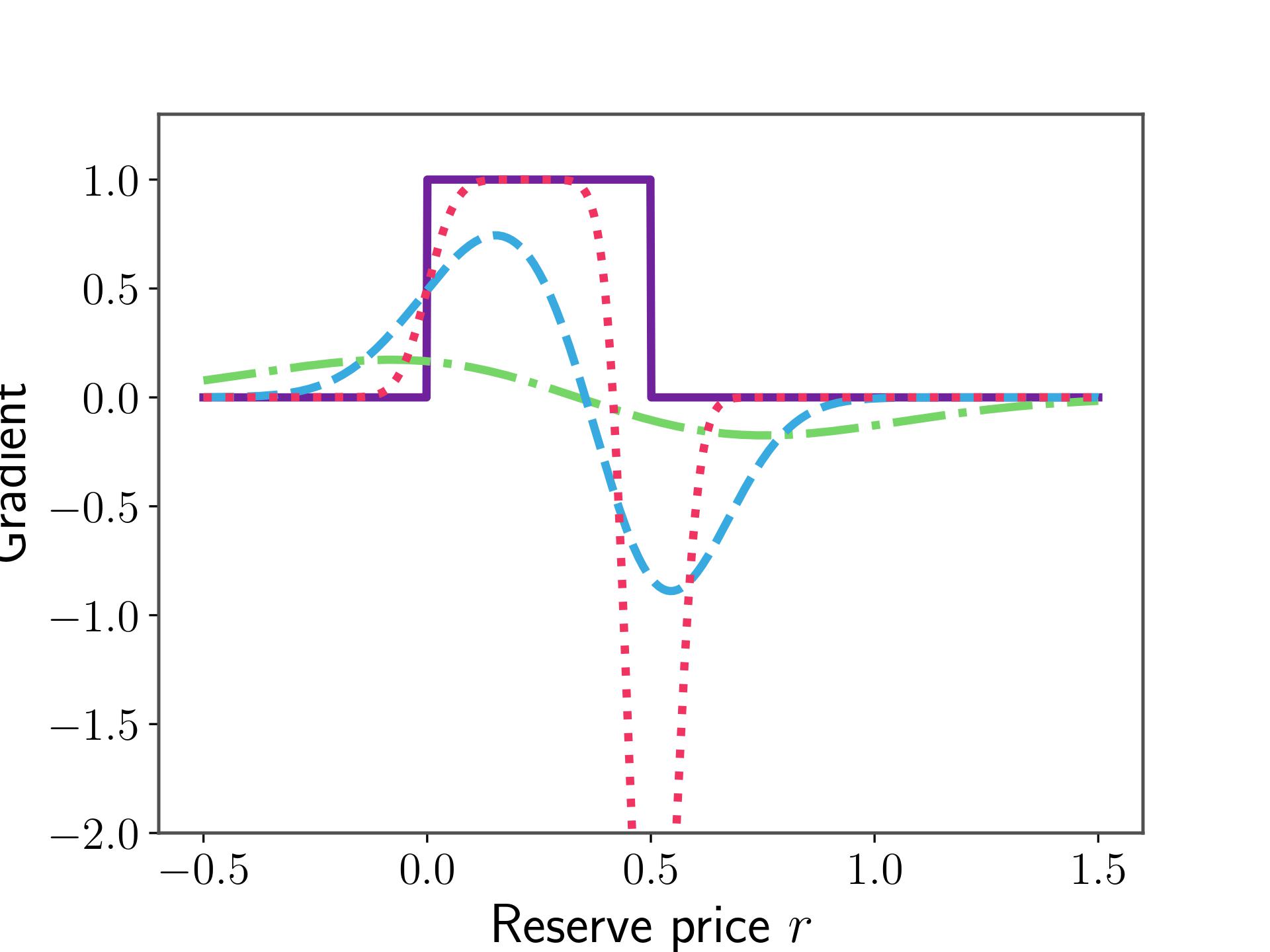
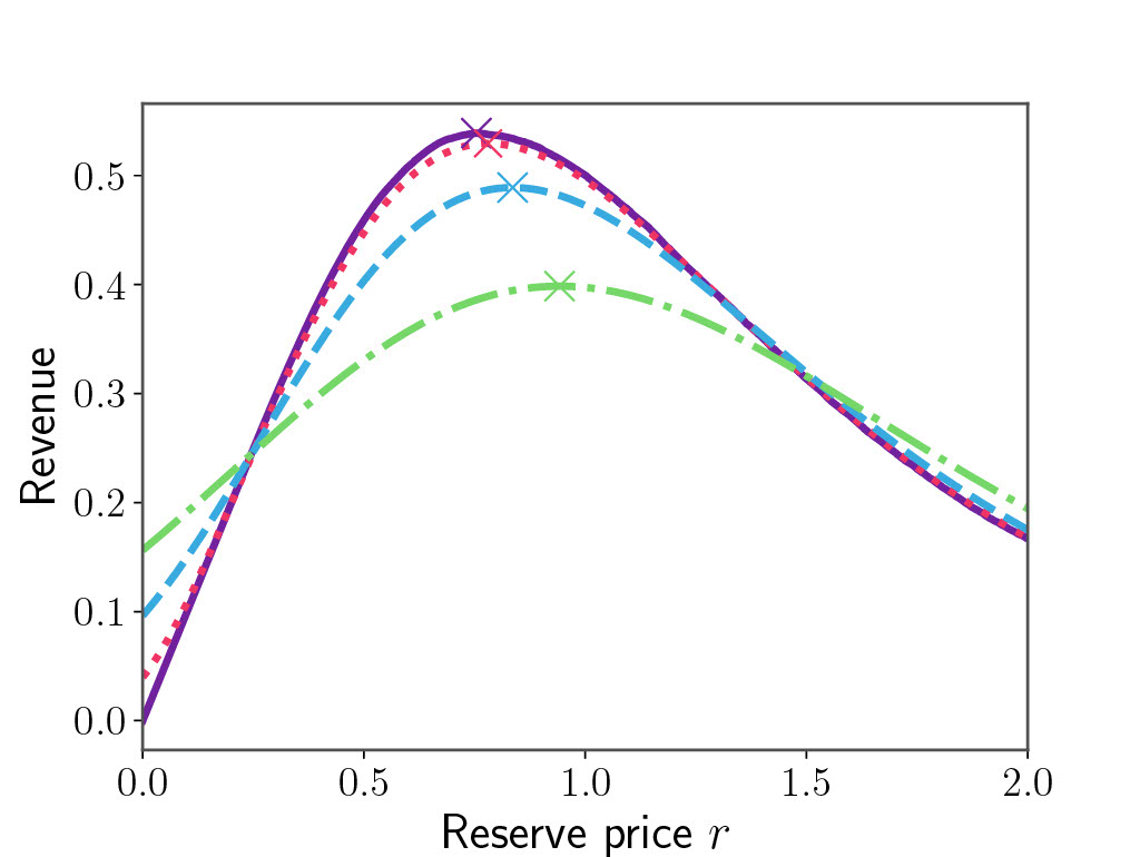
The problem with smoothing is that there is no reason for $\Pi^F$ and $\Pi_k^F$ to have the same minimiser, in other words, \(r^{*}_k \neq r^*\) for $\sigma>0$. So we want $\sigma$ to be as small as possible for the bias \(\vert r^{*}_k - r^*\vert\) to be small, but we also know that the gradient estimate breaks as $\sigma\to 0$. What happens will be clear in Figure 1.

Figure 1. Plots of $\nabla p_k(\cdot,0.5)$ (left) and $\Pi^F_k$ (right) for different valuesIn decreasing order red (dotted), blue (dashed), green (dashed and dotted). of $\sigma$, alongside the ground truths $\1_{r\in(0,0.5)}$ and $\Pi^F$ ( in solid purple).

When $\sigma$ is large the curve is very smooth, and no value of $b$ will lead to a large gradient, which is to say a large change in the iterates $\vert r_{t+1}-r_{t}\vert$. We expect the trajectory of iterates to have very low variance as a consequence, but the bias might be large. Conversely, as the approximation gets better, the gradient of $p_k$ gets arbitrarily large near $r$, which means that a sample landing here can send the iterates very far. In this case, the bias will be very low, since the curves are almost equal, but the variance will be very high.

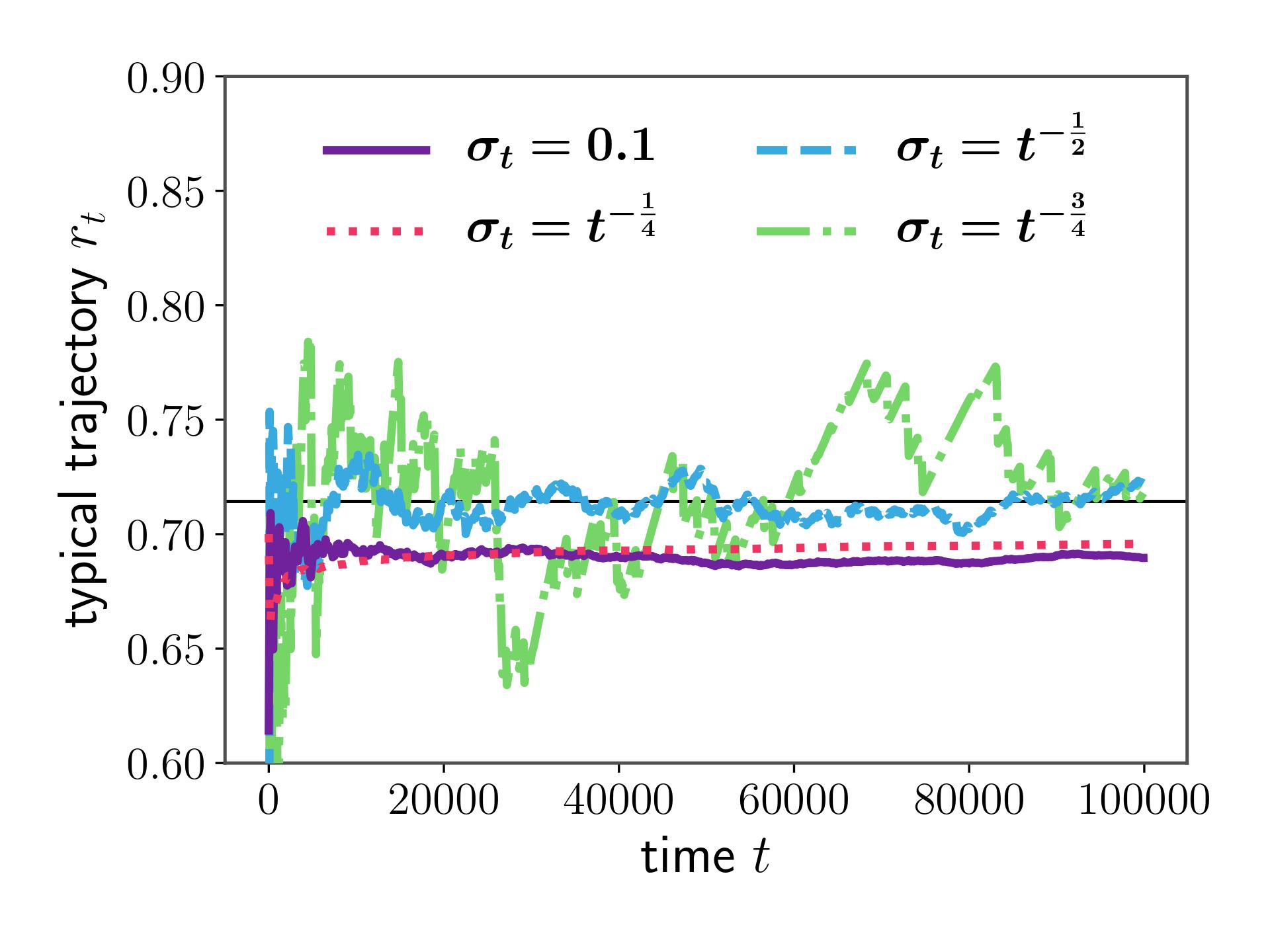
This classical learning theory dilemma is solved by analysing the error $\vert r_t-r^*$ to find how to balance the bias and variance and decrease them both over time at the correct rate. Setting aside the details of the proof, we want to set $\sigma(t)\simeq t^{-\frac12}$ as the schedule for decreasing the variance. You can see in Figure 2. how decreasing $\sigma$ too quickly or too slowly ($t^{-\frac14}$ vs $t^{-\frac34}$) leads to smooth but biased convergence or unbiased but erratic convergence, respectively.

Figure 2. Plots of a sequence of iterates of SG from different decay schemes for $\sigma$, alongside the ground truths $r^*$ (in solid black).

With this choice of $\sigma(t)$ we have therefore designed a method which converges to the optimum and only requires $\Oc(1)$ update cost in time and memory, which answers ii. In the paper, we show that the rate of convergence of this algorithm is $\Oc(t^{-\frac12})$.

Conclusion

In this project, the objective is to propose learning algorithms specifically tailored to auction theoretic problems, with an eye on computational efficiency. This is motivated by the scale at which internet ad auctions are run, which leaves existing methods computationally obsolete.

In we provided the first real-time (constant time and memory update cost) algorithm for learning reserve prices in a (lazy) second-price auction. This algorithm can be run fully online regardless of the frequency of auctions and comes with a convergence guarantee of $\Oc(t^{-\frac12})$. The standard method in the literature comes at a cost of $\Oc(n)$ in time and memory but achieves a rate of $\Oc(t^{-1})$.

All in all, it is surprisingly complicated to sell a bottle of wine properly!

Extensions

The mathematical interest of this problem mostly lies first in unusual probabilistic problems, such as the question over which convolutions preserve some relaxed form of convexity, and second in quantifying computational trade-offs.

In the first vein, we have barely scratched the surface of the problem: other auction formats, strategic bidders, bandit/censored feedback, and more exist to complexify the problem. One key extension which is surprisingly difficult is to turn the bid into a function of some public features $x_t\in\Rb^d$ and try and learn a model of this function. It is non-trivial to extend the convolution method above to this problem since composition does not preserve pseudo-concavity. Following Ibragimov, finding the class of functions which preserves pseudo-concavity by composition should tell us something about which functions preserve the unimodality of random variables, which is doubtless an interesting problem for probabilists.

In the second vein, on the other hand, the tantalising question is whether there is an algorithm which costs only $\Oc(1)$ at each step which achieves the rate $\Oc(t^{-1})$? It might be possible with second-order methods, but the question suggests a notion of convergence hardness under computational constraints which I don’t think I have seen explored before.

However, given some a priori information about $F$, I think it would be possible to find a well-tuned kernel which performs much better than Gaussian. This is suggested by the asymmetry of the problem (because $p$ is highly asymmetrical), which would encourage us to intentionally bias a low variance kernel to counteract its natural bias, for example by using an asymmetrical kernel like a Gumbel distribution. In general, the question of the optimal kernel for a given $F$ might yield interesting insights.